US ECONOMICS

GDP

DoC. BEA.  May 30, 2019. Gross Domestic Product, 1st quarter 2019 (second estimate); Corporate Profits, 1st quarter 2019 (preliminary estimate)

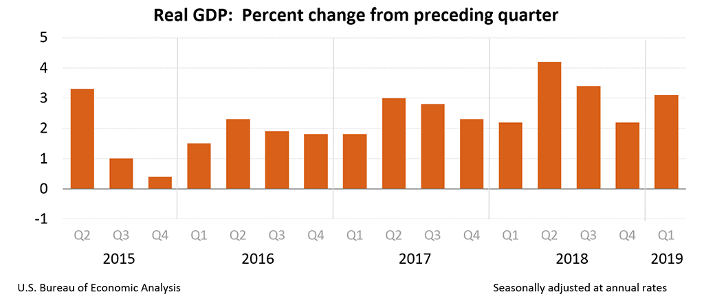
Real gross domestic product (GDP) increased at an annual rate of 3.1 percent in the first quarter of 2019 (table 1), according to the "second" estimate released by the Bureau of Economic Analysis. In the fourth quarter, real GDP increased 2.2 percent.

The GDP estimate released today is based on more complete source data than were available for the "advance" estimate issued last month.  In the advance estimate, the increase in real GDP in the first quarter was 3.2 percent. Today's estimate reflects downward revisions to nonresidential fixed investment and private inventory investment and upward revisions to exports and personal consumption expenditures (PCE). Imports, which are a subtraction in the calculation of GDP, were revised up; the general picture of economic growth remains the same (see "Updates to GDP" on page 2).

Real gross domestic income (GDI) increased 1.4 percent in the first quarter, compared with an increase of 0.5 percent (revised) in the fourth quarter. The average of real GDP and real GDI, a supplemental measure of U.S. economic activity that equally weights GDP and GDI, increased 2.2 percent in the first quarter, compared with an increase of 1.3 percent in the fourth quarter (table 1).

The increase in real GDP in the first quarter reflected positive contributions from PCE, private inventory investment, exports, state and local government spending, and nonresidential fixed investment that were partly offset by a negative contribution from residential fixed investment. Imports, which are a subtraction in the calculation of GDP, decreased (table 2).

The acceleration in real GDP in the first quarter reflected an upturn in state and local government spending, accelerations in private inventory investment and in exports, and a smaller decrease in residential investment. These movements were partly offset by decelerations in PCE and nonresidential fixed investment, and a downturn in federal government spending. Imports turned down.

Current–dollar GDP increased 3.6 percent, or $183.7 billion, in the first quarter to a level of $21.05 trillion. In the fourth quarter, current-dollar GDP increased 4.1 percent, or $206.9 billion (table 1 and table 3).

The price index for gross domestic purchases increased 0.7 percent in the first quarter, compared with an increase of 1.7 percent in the fourth quarter (table 4). The PCE price index increased 0.4 percent, compared with an increase of 1.5 percent. Excluding food and energy prices, the PCE price index increased 1.0 percent, compared with an increase of 1.8 percent.

Updates to GDP

The percent change in first-quarter real GDP was revised down 0.1 percentage point from the advance estimate. Downward revisions to nonresidential fixed investment and private inventory investment and an upward revision to imports were mostly offset by upward revisions to exports and PCE. For more information, see the Technical Note. A detailed "Key Source Data and Assumptions" file is also posted for each release.  For information on updates to GDP, see the "Additional Information" section that follows.

	Advance Estimate	Second Estimate
	(Percent change from preceding quarter)
Real GDP	3.2	3.1
Current-dollar GDP	3.8	3.6
Real GDI	…	1.4
Average of Real GDP and Real GDI	…	2.2
Gross domestic purchases price index	0.8	0.7
PCE price index	0.6	0.4

For the fourth quarter of 2018, the percent change in real GDI was revised from 1.7 percent to 0.5 percent based on newly available fourth-quarter tabulations from the BLS Quarterly Census of Employment and Wages program.

Corporate Profits (table 10)

Profits from current production (corporate profits with inventory valuation and capital consumption adjustments) decreased $65.4 billion in the first quarter, compared with a decrease of $9.7 billion in the fourth quarter.

Profits of domestic financial corporations increased $7.4 billion in the first quarter, in contrast to a decrease of $25.2 billion in the fourth quarter. Profits of domestic nonfinancial corporations decreased $62.1 billion, in contrast to an increase of $13.6 billion. Rest-of-the-world profits decreased $10.7 billion, in contrast to an increase of $1.9 billion. In the first quarter, receipts increased $4.0 billion, and payments increased $14.8 billion.

FULL DOCUMENT: https://www.bea.gov/system/files/2019-05/gdp1q19_2nd.pdf

INTERNATIONAL TRADE

US CENSUS. 05/30/2019. Advance U.S. International Trade in Goods

The advance international trade deficit in goods increased to $72.1 billion in April from $71.9 billion in March as exports decreased more than imports.

• April 2019: 72.1° $ billion
• March 2019: 71.9° $ billion

(*) The 90% confidence interval includes zero. The Census Bureau does not have sufficient statistical evidence to conclude that the actual change is different from zero.

(°) Statistical significance is not applicable or not measurable for these surveys. The Manufacturers’ Shipments, Inventories and Orders estimates are not based on a probability sample, so we can neither measure the sampling error of these estimates nor compute confidence intervals.

(r) Revised.

All estimates are seasonally adjusted except for the Rental Vacancy Rate, Home Ownership Rate, Quarterly Financial Report for Retail Trade, and Quarterly Services Survey. None of the estimates are adjusted for price changes.

FULL DOCUMENT: https://www.census.gov/econ/indicators/advance_report.pdf

DoC. UITC. May 30, 2019. U.S. Department Of Commerce Issues Affirmative Preliminary Antidumping Duty Determination on Aluminum Wire and Cable from China

WASHINGTON – Today, the U.S. Department of Commerce announced the affirmative preliminary determination in the antidumping duty (AD) investigation of imports of aluminum wire and cable from China, finding that that exporters from China have dumped aluminum wire and cable in the United States at a margin of 58.51 to 63.47 percent.

As a result of today’s decision, Commerce will instruct U.S. Customs and Border Protection to collect cash deposits from importers of aluminum wire and cable from China based on the preliminary rates noted above.

In 2017, imports of aluminum wire and cable from China were valued at an estimated $157.2 million.

The petitioners are Encore Wire Corporation (McKinney, TX) and Southwire Company, LLC (Carrollton, GA).

The strict enforcement of U.S. trade law is a primary focus of the Trump Administration. Since the beginning of the current Administration, Commerce has initiated 168 new antidumping and countervailing duty investigations – this is a 223 percent increase from the comparable period in the previous administration.

Antidumping and countervailing duty laws provide American businesses and workers with an internationally accepted mechanism to seek relief from the harmful effects of the unfair pricing of imports into the United States. Commerce currently maintains 482 antidumping and countervailing duty orders which provide relief to American companies and industries impacted by unfair trade.

Commerce is scheduled to announce the final determination on or about October 9, 2019.

If Commerce’s final determination is affirmative, the U.S. International Trade Commission (ITC) will be scheduled to make its final injury determination on or about November 22, 2019. If Commerce makes an affirmative final determination of dumping, and the ITC makes an affirmative final injury determination, Commerce will issue an AD order. If Commerce makes a negative final determination of dumping, or the ITC makes a negative final determination of injury, the investigation will be terminated and no orders will be issued.

The U.S. Department of Commerce’s Enforcement and Compliance unit within the International Trade Administration is responsible for vigorously enforcing U.S. trade law and does so through an impartial, transparent process that abides by international law and is based on factual evidence provided on the record.

Foreign companies that price their products in the U.S. market below the cost of production or below prices in their home markets are subject to antidumping duties. Companies that receive unfair subsidies from their governments, such as grants, loans, equity infusions, tax breaks, or production inputs, are subject to countervailing duties aimed at directly countering those subsidies.

Fact sheet: https://enforcement.trade.gov/download/factsheets/factsheet-prc-aluminum-wire-cable-ad-prelim-053019.pdf

DoC. USITC. May 29, 2019. U.S. Department of Commerce Issues Affirmative Preliminary Antidumping Duty Determination on Mattresses from China

WASHINGTON – Today, the U.S. Department of Commerce announced the affirmative preliminary determination in the antidumping duty (AD) investigation of imports of mattresses from China, finding that exporters from China have dumped mattresses in the United States at margins ranging from 38.56 to 1,731.75 percent.

As a result of today’s decisions, Commerce will instruct U.S. Customs and Border Protection to collect cash deposits from importers of mattresses from China based on the preliminary rates noted above.

In 2017, imports of mattresses from China were valued at an estimated $436.5 million.

The petitioners are Corsicana Mattress Company (Dallas, TX), Elite Comfort Solutions (Newman, GA), Future Foam Inc. (Council Bluffs, IA), FXI Inc. (Media, PA), Innocor, Inc. (Red Bank, NJ), Kolcraft Enterprises Inc. (Chicago, IL), Leggett & Platt, Incorporated (Carthage, MO), Serta Simmons Bedding, LLC (Atlanta, GA), and Tempur Sealy International, Inc. (Lexington, KY).

The strict enforcement of U.S. trade law is a primary focus of the Trump Administration. Since the beginning of the current Administration, Commerce has initiated 168 new antidumping and countervailing duty investigations – this is a 223 percent increase from the comparable period in the previous administration.

Antidumping and countervailing duty laws provide American businesses and workers with an internationally accepted mechanism to seek relief from the harmful effects of the unfair pricing of imports into the United States. Commerce currently maintains 481 antidumping and countervailing duty orders which provide relief to American companies and industries impacted by unfair trade.

Commerce is scheduled to announce the final determinations on or about October 11, 2019.

If Commerce’s final determinations are affirmative, the U.S. International Trade Commission (ITC) will be scheduled to make its final injury determinations on or about November 24, 2019. If Commerce makes affirmative final determinations of dumping, and the ITC makes affirmative final injury determinations, Commerce will issue AD orders. If Commerce makes negative final determinations of dumping, or the ITC makes negative final determinations of injury, the investigations will be terminated and no orders will be issued.

The U.S. Department of Commerce’s Enforcement and Compliance unit within the International Trade Administration is responsible for vigorously enforcing U.S. trade law and does so through an impartial, transparent process that abides by international law and is based on factual evidence provided on the record.

Foreign companies that price their products in the U.S. market below the cost of production or below prices in their home markets are subject to antidumping duties. Companies that receive unfair subsidies from their governments, such as grants, loans, equity infusions, tax breaks, or production inputs, are subject to countervailing duties aimed at directly countering those subsidies.

Fact sheet:
https://enforcement.trade.gov/download/factsheets/factsheet-prc-mattresses-ad-prelim-052919.pdf

DoS. USITC. May 29, 2019. U.S. Department Of Commerce Issues Affirmative Preliminary Antidumping Duty Determinations on Refillable Stainless Steel Kegs from China, Germany, and Mexico

WASHINGTON – Today, the U.S. Department of Commerce announced the affirmative preliminary determinations in the antidumping duty (AD) investigations of imports of refillable stainless steel kegs from China, Germany, and Mexico, finding that exporters from China, Germany, and Mexico have dumped refillable stainless steel kegs in the United States at the following rates:

• China – 2.01 to 79.71 percent
• Germany – 8.61 percent
• Mexico – 18.48 percent

As a result of today’s decisions, Commerce will instruct U.S. Customs and Border Protection to collect cash deposits from importers of refillable stainless steel kegs from China, Germany, and Mexico based on the preliminary rates noted above.

In 2017, imports of refillable stainless steel kegs from China, Germany, and Mexico were valued at an estimated $18.1 million, $11.8 million, and $5.7 million, respectively.

The petitioner is American Keg Company, LLC (Pottstown, PA).

The strict enforcement of U.S. trade law is a primary focus of the Trump Administration. Since the beginning of the current Administration, Commerce has initiated 168 new antidumping and countervailing duty investigations – this is a 223 percent increase from the comparable period in the previous administration.

Antidumping and countervailing duty laws provide American businesses and workers with an internationally accepted mechanism to seek relief from the harmful effects of the unfair pricing of imports into the United States. Commerce currently maintains 481 antidumping and countervailing duty orders which provide relief to American companies and industries impacted by unfair trade.

Commerce is scheduled to announce the final determination on or about August 13, 2019 with respect to Mexico and on or about October 16, 2019 with respect to China and Germany.

If Commerce’s final determinations are affirmative, the U.S. International Trade Commission (ITC) will be scheduled to make its final injury determination on or about September 26, 2019 for Mexico and on or about November 29, 2019 for China and Germany. If Commerce makes affirmative final determinations of dumping, and the ITC makes affirmative final injury determinations, Commerce will issue AD orders. If Commerce makes negative final determinations of dumping, or the ITC makes negative final determinations of injury, the investigations will be terminated and no orders will be issued.

The U.S. Department of Commerce’s Enforcement and Compliance unit within the International Trade Administration is responsible for vigorously enforcing U.S. trade law and does so through an impartial, transparent process that abides by international law and is based on factual evidence provided on the record.

Foreign companies that price their products in the U.S. market below the cost of production or below prices in their home markets are subject to antidumping duties. Companies that receive unfair subsidies from their governments, such as grants, loans, equity infusions, tax breaks, or production inputs, are subject to countervailing duties aimed at directly countering those subsidies.

Fact sheet: https://enforcement.trade.gov/download/factsheets/factsheet-multiple-refillable-stainless-steel-kegs-ad-prelim-052919.pdf

DoS. USITC. May 29, 2019. U.S. Department of Commerce Initiates Antidumping Duty and Countervailing Duty Investigations of Imports of Certain Quartz Surface Products from India and Turkey

WASHINGTON – Today, the U.S. Department of Commerce announced the initiation of new antidumping duty (AD) and countervailing duty (CVD) investigations to determine whether certain quartz surface products from India and Turkey are being dumped in the United States and to determine if producers in India and Turkey are receiving unfair subsidies.

These antidumping and countervailing duty investigations were initiated based on petitions filed by Cambria Company LLC (Eden Prairie, MN).

The alleged dumping margins are 323.12 percent for India and 85.71 percent for Turkey.

There are 35 subsidy programs alleged for India, including export subsidies, tax programs, grants, loan subsidies, and the provision of goods for less than adequate remuneration. Additionally, there are 23 subsidy programs alleged for Turkey, including tax programs, export credit programs, investment incentive programs, and regional development subsidies.

If Commerce makes affirmative findings in these investigations, and if the U.S. International Trade Commission (ITC) determines that dumped and/or unfairly subsidized U.S. imports of quartz surface products from India and Turkey are causing injury to the U.S. industry, Commerce will impose duties on those imports in the amount of dumping and/or unfair subsidization found to exist.

In 2018, imports of quartz surface products from India and Turkey were valued at an estimated $69.5 million and $28 million, respectively.

Next Steps:

During Commerce’s investigations into whether quartz surface products from India and Turkey are being dumped and/or unfairly subsidized, the ITC will conduct its own investigations into whether the U.S. industry and its workforce are being harmed by such imports. The ITC will make its preliminary determinations on or before June 24, 2019. If the ITC preliminarily determines that there is injury or threat of injury, then Commerce’s investigations will continue, with the preliminary CVD determination scheduled for August 1, 2019, and preliminary AD determination scheduled for October 15, 2019, unless these deadlines are extended.

If Commerce preliminarily determines that dumping and/or unfair subsidization is occurring, then it will instruct U.S. Customs and Border Protection to start collecting cash deposits from all U.S. companies importing quartz surface products from India and Turkey.

Final determinations by Commerce in these cases are scheduled for October 15, 2019, for the CVD investigation, and December 30, 2019, for the AD investigation, but those dates may be extended. If Commerce finds that products are not being dumped and/or unfairly subsidized, or the ITC finds in its final determinations there is no harm to the U.S. industry, then the investigations will be terminated and no duties will be applied.

The strict enforcement of U.S. trade law is a primary focus of the Trump Administration. Since the beginning of the current Administration, Commerce has initiated 168 new antidumping and countervailing duty investigations – this is a 223 percent increase from the comparable period in the previous administration.

Antidumping and countervailing duty laws provide American businesses and workers with an internationally accepted mechanism to seek relief from the harmful effects of the unfair pricing of imports into the United States. Commerce currently maintains 481 antidumping and countervailing duty orders which provide relief to American companies and industries impacted by unfair trade.

The U.S. Department of Commerce’s Enforcement and Compliance unit within the International Trade Administration is responsible for vigorously enforcing U.S. trade law and does so through an impartial, transparent process that abides by international law and is based on factual evidence provided on the record.

Foreign companies that price their products in the U.S. market below the cost of production or below prices in their home markets are subject to antidumping duties. Companies that receive unfair subsidies from their governments, such as grants, loans, equity infusions, tax breaks, or production inputs, are subject to countervailing duties aimed at directly countering those subsidies.

Fact sheet: https://enforcement.trade.gov/download/factsheets/factsheet-multiple-quartz-surface-products-initiation-052919.pdf

MONETARY POLICY

FED. May 30, 2019. Speech. Monetary Policy and Financial Stability. Vice Chair for Supervision Randal K. Quarles. At "Developments in Empirical Macroeconomics," a research conference sponsored by the Federal Reserve Board and the Federal Reserve Bank of New York, Washington, D.C.

Thank you for the opportunity to take part in today's "Developments in Empirical Macroeconomics" conference. I would like to use my time here to talk about a topic of interest to many central bankers and macroeconomists: the interaction of monetary policy and financial stability. As you well know, monetary policy has powerful effects on financial markets, the financial system, and the broader economy. Conversely, financial instability, by impairing the provision of credit and other financial services, can depress economic growth, cause job losses, and push inflation too low. Accordingly, financial stability, through its effects on the Federal Reserve's dual-mandate goals of maximum employment and stable prices, must be a consideration in the setting of monetary policy.

Against this backdrop, a natural—yet quite complex—question is whether monetary policy should be used to promote financial stability. This question is hotly debated in a large and growing academic literature, and any serious answer has to be subject to considerable nuance. At the same time, my sense is that the balance is clearly tilted toward the conclusion that macroprudential policies—through-the-cycle resilience, stress tests, and the countercyclical capital buffer (CCyB)—may be better targeted to promoting financial stability than monetary policy.1

Before I wade into the lessons from past research and experience, I would like to highlight that this question is not just academic. As you know, the economy, monetary policy, and financial stability are intertwined. For example, the past three recessions were preceded by some combination of elevated asset prices, rapid increases in borrowing by businesses and households, and excessive risk-taking in the financial sector. These financial vulnerabilities have amplified adverse shocks to the overall economy time and again. Such concerns have resurfaced among some observers, as the current long expansion has brought business borrowing to new heights. My own assessment is that even though business debt is elevated, at least by some measures, overall financial stability risks are not, as the financial sector has substantial loss-absorbing capacity and is not overly reliant on unstable short-term funding. Yet, even if the risk of financial system disruption does not seem high, it well remain true that if the economy weakens, some businesses may default on this debt, potentially leading to a contraction in investment, a slow-down in hiring, and possibly to an unusual tightening in financial conditions. These concerns highlight how cyclical factors influencing monetary policy borrowers may overlap with financial stability considerations.

How Monetary Policy Can Influence Financial Stability

Let me begin by laying out how monetary policy can influence financial stability. Monetary policy, operating primarily through adjustments in the level of short-term interest rates, has powerful effects on the entire financial system. A more accommodative monetary policy lowers interest rates across the maturity spectrum. The textbook result is that mortgage rates and corporate borrowing rates, among others, decline; equity prices rise; and the dollar exchange rate depreciates. In other words, financial conditions broadly ease, spurring households to buy more and businesses to invest and hire, thereby supporting economic growth and price stability.2

Monetary policy, however, if too accommodative, may lead to a buildup of financial vulnerabilities. These incentives arrive through a number of channels. For instance, low interest rates reduce the cost of borrowing, and so may prompt businesses and households to overborrow. Low rates may lead to a speculative bubble by compressing risk premiums for assets—such as equity, corporate bonds, and housing—and potentially leading investors to extrapolate price gains into the future in a bout of irrational exuberance. Low rates may also squeeze the profitability of financial intermediaries through narrow interest margins and other factors. In turn, these intermediaries as well as investors that had promised fixed nominal rates of return—such as insurance companies and pension funds—may "reach for yield," or take on more credit or duration risk in their portfolios in order to maintain high returns. Taken to extremes, this story often does not end well. Periods of excessive leverage, rapid credit growth, or buoyant credit market sentiment increase the risk to economic growth.3

These dynamics point to the possibility that accommodative monetary policy, while necessary to support activity during the early stages of an economic expansion, may also increase vulnerabilities in the financial system, especially if maintained for too long. These vulnerabilities weaken the financial system's ability to absorb negative shocks, and so when a shock arrives, losses mount, the financial system weakens, lending slows, and economic activity slows by more than it would have otherwise, potentially leading to an economic downturn or a more severe recession.

Should Financial Vulnerabilities Affect the Stance of Monetary Policy?

These observations lead to the important question of whether and how financial vulnerabilities should affect the setting of monetary policy. One simple framework for evaluating the tradeoffs associated with actively setting monetary policy to lean against the buildup of financial vulnerabilities is to examine the costs and benefits of such a policy in terms of unemployment and inflation. In this approach, the costs of tightening monetary policy in response to a buildup of financial vulnerabilities are lower employment and potentially below target inflation in the near term. The benefits are possibly reducing the risk of a future financial crisis, an event likely associated with a much larger fall in employment and inflation.

One view is that monetary policy curbs household and business borrowing only modestly but can boost the unemployment rate notably. And so using monetary policy to damp borrowing does more harm than good. According to this view, using monetary policy to lean against financial vulnerabilities does not generate significant net benefits and may be counterproductive—increasing unemployment and decreasing inflation below a desired level with little reduction in risks to financial stability.4

At the same time, some research has identified circumstances under which the benefits of using monetary policy to lean against financial vulnerabilities could outweigh the costs.5 A key consideration is the estimated amount of economic activity lost in a financial crisis—and some research suggests such losses may be quite large, which raises the benefits of leaning against imbalances. Similarly, monetary policy may affect a broad range of financial imbalances—excessively high house or equity prices and leverage within the financial sector—and the full set of these effects could shift the risk of financial instability sufficiently, at least under some circumstances, to make leaning against financial vulnerabilities with monetary policy desirable. The broader point is that we do not fully understand the cost–benefit tradeoff and whether monetary policy adjustments for financial stability reasons may be appropriate at some times.

Whither Macroprudential Policy?

Of course, there is one additional and critical factor to consider when weighing adjustments to the stance of monetary policy for financial stability reasons: the availability and efficacy of other instruments to promote financial stability. After all, the pursuit of multiple goals—full employment, price stability, and financial stability, for example—likely requires multiple tools. This is just common sense. Economists have a name for this common-sense notion: the Tinbergen principle.

Effective supervisory, regulatory, and macroprudential policy tools appear to be well placed to address financial vulnerabilities. In particular, these tools may be used to increase the resilience of the financial sector against a broad range of adverse shocks and, perhaps, lean against the buildup of specific financial vulnerabilities. At the Federal Reserve, we have emphasized a set of structural, or through-the-cycle, regulatory and supervisory policies as our primary macroprudential tools to promote financial stability. These measures include strong capital and liquidity requirements for banks, especially the largest and most systemic institutions. In addition, our supervisory stress tests evaluate the ability of large banks to weather severe economic stress and the failure of their largest counterparty as well as examining the risk‑management practices of the firms. Moreover, the stress-test scenarios are designed to generally be more severe during buoyant economic periods when vulnerabilities may build. Furthermore, our stress tests consider the potential effects of specific risks we have identified in our financial stability monitoring work. For example, the tests in recent years have included hypothetical severe strains in corporate debt markets, exploring the resilience of the participating banks to the risks associated with the increase in business borrowing.

In addition, the Federal Reserve monitors a wide range of indicators for signs of potential risks to financial stability that may merit a policy response, and we now publish a summary of this monitoring in our semiannual Financial Stability Report. If vulnerabilities are identified as being meaningfully above normal, the Federal Reserve can require large banks to increase their loss-absorbing capacity through increases in the CCyB.6

Despite all of these efforts, we understand that these tools have limitations. First, central bankers' experience with macroprudential tools, including the CCyB, is limited. Second, regulation and macropudential tools can reduce economic efficiency and hamper economic growth by limiting the ability of the market to allocate financial resources. For this reason, the Federal Reserve has been evaluating ways in which our supervisory and financial stability goals can be achieved more efficiently, and it has been participating in global efforts to evaluate the effects of reforms under the auspices of the Financial Stability Board. Third, macroprudential policies that are targeted to banks may create an incentive for financial intermediation to migrate outside of the regulated banking system. The vulnerabilities may still emerge, albeit elsewhere in the financial system—perhaps in institutions or structures that are less stable and resilient than our banks. In part reflecting these incentives, we regularly monitor financial intermediation both inside and outside of the banking system.

Summary

To sum up, while there is evidence that financial vulnerabilities have the potential to translate into macroeconomic risks, a general consensus has emerged that monetary policy should be guided primarily by the outlook for unemployment and inflation and not by the state of financial vulnerabilities. Financial system resilience, supported by strong through-the-cycle regulatory and supervisory policies, remains a key defense against financial system and macroeconomic shocks.

There is a clear need for new theory and empirics to address the questions about monetary policy and financial stability I have posed today. I encourage you to continue to contribute to these answers. By engaging the help of the wider academic community, conferences such as this one provide an invaluable opportunity to make progress on issues of great importance for economic policy.

References

• Adrian, Tobias, Nina Boyarchenko, and Domenico Giannone (2019). "Vulnerable Growth," American Economic Review, vol. 109 (April), pp. 1263–89.
• Adrian, Tobias, and Nellie Liang (2018). "Monetary Policy, Financial Conditions, and Financial Stability," International Journal of Central Banking, vol. 14 (January), pp. 73–131.
• Ajello, Andrea, Thomas Laubach, David López-Salido, and Taisuke Nakata (2019). "Financial Stability and Optimal Interest Rate Policy," International Journal of Central Banking, vol. 15 (March), pp. 279–326.
• Bernanke, Ben S., and Mark Gertler (1995). "Inside the Black Box: The Credit Channel of Monetary Policy Transmission," Journal of Economic Perspectives, vol. 9 (Fall), pp. 27–48.
• Boivin, Jean, Michael T. Kiley, and Frederic S. Mishkin (2010). "How Has the Monetary Transmission Mechanism Evolved over Time?" in Benjamin M. Friedman and Michael Woodford, eds., Handbook of Monetary Economics, 1st ed., vol. 3. Amsterdam: Elsevier, pp. 369–442.
• Gourio, Francois, Jae W. Sim, and Anil K. Kashyap (2018). "The Trade Offs in Leaning against the Wind," IMF Economic Review, vol. 66 (March), pp. 70–115.
• Kiley, Michael T. (2018). "Unemployment Risk (PDF)," Finance and Economics Discussion Series 2018-067. Washington: Board of Governors of the Federal Reserve System, September.
• López-Salido, David, Jeremy C. Stein, and Egon Zakrajšek (2017). "Credit-Market Sentiment and the Business Cycle," Quarterly Journal of Economics, vol. 132 (August), pp. 1373–1426.
• Mian, Atif, Amir Sufi, and Emil Verner (2017). "Household Debt and Business Cycles Worldwide," Quarterly Journal of Economics, vol. 132 (November), pp. 1755–1817.
• Schularick, Moritz, and Alan M. Taylor (2012). "Credit Booms Gone Bust: Monetary Policy, Leverage Cycles, and Financial Crises, 1870–2008," American Economic Review, vol. 102 (April), pp. 1029–61.
• Svensson, Lars E.O. (2014). "Inflation Targeting and 'Leaning against the Wind,'" International Journal of Central Banking, vol. 10 (June), pp. 103–114.
• ——— (2017). "Cost–Benefit Analysis of Leaning against the Wind," Journal of Monetary Economics, vol. 90 (October), pp. 193–213.

Notes

1. These remarks represent my own views, which do not necessarily represent those of the Federal Reserve Board or the Federal Open Market Committee.
2. For reviews of the various monetary policy transmission channels to the real economy, see Bernanke and Gertler (1995) and Boivin, Kiley, and Mishkin (2010).
3. See, among others, Schularick and Taylor (2012); López-Salido, Stein, and Zakrajsek (2017); Mian, Sufi, and Verner (2017); Adrian, Boyarchenko, Giannone (2019); and Kiley (2018).
4. See, for instance, Svensson (2014, 2017).
5. See, for example, Ajello, Laubach, López-Salido, and Nakata (2018); Guorio, Sim, and Kashyap (2018); and Adrian and Liang (2018).
6. CCyB also builds financial-sector resilience during periods when financial vulnerabilities are high and there is a risk of potential losses within the banking sector that could strain the supply of credit. Furthermore, the CCyB might be a more effective tool than monetary policy to mitigate financial vulnerabilities, as the benefits are comparable to those of using monetary policy while the costs are an order of magnitude smaller.

EMPLOYMENT

FED. May 30, 2019. Speech. Sustaining Maximum Employment and Price Stability. Vice Chair Richard H. Clarida. At the Economic Club of New York, New York, New York

Thank you for that generous introduction. I have attended Economic Club of New York events many times over the years and have always enjoyed the programs that feature engaging speakers sharing important insights on timely topics. It is a distinct honor to appear before you today from this side of the podium, and I do hope my remarks will contribute to this proud tradition.1

In July, the current U.S. economic expansion will become the longest on record—or at least the record since the 1850s, which is as far back as the National Bureau of Economic Research tracks U.S. business cycles.2 In anticipation of that milestone, I would like to take stock of where the U.S. economy is today, to assess its future trajectory, to review some important structural changes in the economy that have occurred over the past decade, and to explore what all of this might mean for U.S. monetary policy.

The Federal Reserve has a specific mandate assigned to it in statute by the Congress, which is the dual mandate of maximum employment and price stability. As I speak today, the economy is as close to achieving both legs of this dual mandate as it has been in 20 years. My colleagues and I understand that our responsibility is to conduct a monetary policy that not only is supportive of and consistent with achieving maximum employment and price stability, but also, once achieved, is appropriate, nimble, and consistent with sustaining maximum employment and price stability for as long as possible. And thus, the title of my talk today is "Sustaining Maximum Employment and Price Stability."

Midway through the second quarter of 2019, the U.S. economy is in a good place. Over the past four quarters, gross domestic product (GDP) growth has averaged 3.2 percent, which compares with an average growth rate of 2.3 percent since the recovery began in the summer of 2009. By most estimates, fiscal policy played an important role in boosting growth in 2018, and I expect that fiscal policies will continue to support growth in 2019. Over the same four quarters, the unemployment rate has averaged 3.8 percent, and the most recent reading, at 3.6 percent, is near its lowest level in 50 years. Moreover, average monthly job gains have continued to outpace the increases needed to provide jobs for new entrants to the labor force. Wages have been rising broadly in line with productivity and prices and thus, at present, do not signal rising cost-push pressure. Notwithstanding strong growth and low unemployment, U.S. inflation remains muted—currently, it is somewhat below our 2 percent longer-run objective for the personal consumption expenditures (PCE) price deflator—and inflation expectations, according to a variety of measures, continue to be stable.

As we look ahead, in our March Summary of Economic Projections, the median projection of Federal Open Market Committee (FOMC) participants was for GDP growth of around 2 percent as the modal, or most likely, outcome over the next three years, for PCE inflation to rise to 2 percent, and for the unemployment rate to edge up to 3.9 percent by 2021.

Before I discuss the outlook for monetary policy, allow me to review some important structural changes that have taken place in the economy over the past decade that will be particularly relevant for our monetary policy decisions.

Structural Changes in the U.S. Economy: Demand and Supply

Perhaps the most significant structural change relevant to monetary policy is that the real, or inflation-adjusted, rate of interest consistent with full employment and price stability, often referred to as the neutral rate, or r*, appears to have fallen in the United States and abroad from more than 2 percent before the crisis to less than 1 percent today.3 The decline in neutral policy rates likely reflects several factors, including aging populations, higher private saving, a greater demand for safe assets, and a slowdown in global productivity growth. The policy implications of the decline in neutral rates are important. All else being equal, a lower neutral rate increases the likelihood that a central bank's policy rate will reach its effective lower bound in a future economic downturn. Such a development, in turn, could make it more difficult during a future downturn for monetary policy to provide sufficient accommodation to rapidly return employment and inflation to mandate-consistent levels.4

Another important potential change in the U.S. economy has been the steady decline in estimates of the structural rate of unemployment consistent with "maximum" employment, often referred to as u*. This decline in u* may be due in part to higher educational attainment and a larger proportion of older workers in the workforce today relative to the workforce of past decades.5 If u* is lower than historical estimates suggest, this would imply that, even with today's historically low unemployment rate, the labor market would not be as tight—and inflationary pressures would not be as strong—as one would expect, based on historical estimates of u*. Indeed, I believe the range of plausible estimates for u* may extend to 4 percent or even below.

I also note that the decline in the unemployment rate in recent years has been accompanied by a pronounced increase in labor force participation for individuals in their prime working years.6 It has also been accompanied since 2014 by a rise in labor's share of national income. As I have documented previously, in the past several U.S. business cycles, labor's share has risen as those expansions proceeded because workers command higher wages in a stronger labor market; notably, in those cycles, the rise in labor's share did not pass through to faster price inflation.7 The previously mentioned increase in prime-age labor force participation has provided employers with a source of additional labor input and has been one factor restraining inflationary pressures. Notwithstanding these recent gains, prime-age participation rates remain somewhat below levels achieved in the 1990s and may still have some more room to run. If so, then potential output could be higher than many current estimates suggest.

Over the past few years, we have also seen evidence of a pickup in U.S. productivity growth, albeit from the very depressed average pace that prevailed throughout most of the expansion. Indeed, as of the first quarter of this year, productivity in the nonfarm business sector rose 2.4 percent over the previous four quarters, its fastest pace since 2010 when the U.S. economy was coming out of the Great Recession. By contrast, in both the 2001–07 and 1982–90 economic expansions, productivity growth was actually slowing relative to its average pace during those expansions. That said, while identifying inflection points in trend productivity growth in real time is notoriously difficult, a pickup in trend productivity growth relative to the pace that prevailed earlier in the expansion is a possibility that we should not, I believe, dismiss.8

Another structural change relevant for monetary policy is that price inflation appears less responsive to resource slack than it did in the past. That is, the short-run price Phillips curve appears to have flattened, implying a change in the dynamic relationship between inflation and employment.9 A flatter Phillips curve is, in a sense, a proverbial double-edged sword. It permits the Federal Reserve to support employment more aggressively during downturns—as was the case during and after the Great Recession—because a sustained inflation breakout is less likely when the Phillips curve is flatter.10 However, a flatter Phillips curve also increases the cost, in terms of economic output, of reversing unwelcome increases in longer-run inflation expectations. Thus, a flatter Phillips curve makes it all the more important that longer-run inflation expectations remain anchored at levels consistent with our 2 percent inflation objective.11

Textbook macroeconomics teaches us that understanding the economy and getting monetary policy right requires that we do our best to understand if—and if so, how—the forces of aggregate demand and supply are evolving relative to historical experience and the predictions of our models. While predicting the future is difficult, with available data it appears that in 2018 and in the first quarter of 2019, the supply side of the economy—employment, participation, and productivity—expanded faster than most forecasters outside and inside the Fed expected. Notwithstanding robust growth in demand over these five quarters, PCE price inflation fell somewhat short of the Fed's 2 percent objective. With this background, let me now turn to the outlook for U.S. monetary policy.

Monetary Policy

As I mentioned earlier, my colleagues and I on the FOMC understand that our priority today is to put in place policies that will help sustain maximum employment and price stability in an economy that appears to be operating close to both of our dual-mandate objectives. In our most recent statements, we have indicated that "the Committee will be patient as it determines what future adjustments to the...federal funds rate may be appropriate to support" our dual-mandate objectives.12 What does this mean in practice? To me, it means that we should allow the data on the U.S. economy to flow in and inform our future decisions.

I believe that the path for the federal funds rate should be data dependent in two distinct ways.13 Monetary policy should be data dependent in the sense that incoming data reveal at any point in time where the economy is relative to the ultimate objectives of price stability and maximum employment. This information on where the economy is relative to the goals of monetary policy is an important input into interest rate feedback rules. Data dependence in this sense is well understood, as it is of the type implied by a large family of policy rules, including Taylor-type rules, in which the parameters of the economy needed to formulate such rules are taken as known.

But, of course, key parameters needed to formulate such rules, including u* and r*, are unknown. As a result, in the real world, monetary policy should be—and in the United States, I believe, is—data dependent in a second sense: Policymakers should and do study incoming data and use models to extract signals that enable them to update and improve estimates of r* and u*. Consistent with my earlier discussion, in the Summary of Economic Projections, FOMC participants have, over the past seven years, repeatedly revised down their estimates of both u* and r* as unemployment fell and real interest rates remained well below previous estimates of neutral without the rise in inflation those earlier estimates would have predicted. And these revisions to u* and r* appeared to have had an important influence on the path for the policy rate actually implemented in recent years.

In addition to u* and r*, another important input into any monetary policy assessment is the state of inflation expectations. Indeed, I believe price stability requires that not only actual inflation be centered at our 2 percent objective, but also that expected inflation be equal to our 2 percent inflation objective. Unlike realized inflation, inflation expectations themselves are not directly observable; they must be inferred from econometric models, market prices, and surveys of households and firms. As I assess the totality of the evidence, I judge that, at present, indicators suggest that longer-term inflation expectations sit at the low end of a range that I consider consistent with our price-stability mandate.

Where does this leave us today? As I already noted, the U.S. economy is in a very good place, with the unemployment rate near a 50-year low, inflationary pressures muted, expected inflation stable, and GDP growth solid and projected to remain so. Moreover, the federal funds rate is now in the range of estimates of its longer-run neutral level, and the unemployment rate is not far below many estimates of u*. Plugging these inputs into a 1993 Taylor-type rule produces a federal funds rate between 2.25 and 2.5 percent, which is the range for the policy rate that the FOMC has reaffirmed since our January meeting. Most recently, the Committee judged at our May meeting that the current stance of policy remains appropriate, and that decision reflects our view that some of the softness in recent inflation data will prove to be transitory. This judgment aligns with some private-sector forecasts, which now project PCE inflation to return to 2 percent by 2020. However, if the incoming data were to show a persistent shortfall in inflation below our 2 percent objective or were it to indicate that global economic and financial developments present a material downside risk to our baseline outlook, then these are developments that the Committee would take into account in assessing the appropriate stance for monetary policy.

Monetary Policy Implementation and Balance Sheet​ Decisions 

Since the beginning of the year, the FOMC has made several important decisions about how it will implement monetary policy and how it will conclude the process of normalizing the size of its balance sheet. These decisions have been made over several meetings and have been part of an ongoing process of the Committee's deliberations. Please allow me to summarize them now.

The FOMC decided at its January meeting to continue to implement monetary policy in a regime with an ample supply of reserves—a regime often referred to as a floor system.14 Such a system, which has been in place since late 2008, does not require the active management of reserves through daily open market operations. Instead, with an ample level of reserves in the banking system, the effective federal funds rate will settle at or slightly above the rate of interest paid on excess reserves (IOER).15 This system has proven to be an efficient means of controlling the policy rate and effectively transmitting the stance of policy to a wide array of other money market instruments and to broader financial conditions. The FOMC continues to view the target range for the federal funds rate as its primary means of adjusting and communicating the stance of monetary policy, although in doing so, we must and do take into account how our balance sheet size, composition, and trajectory impact broader financial conditions. And as we stated in January, although adjustments in the target range for the federal funds rate are our primary tool for adjusting the stance of monetary policy, we are prepared to adjust the details of the plans for balance sheet normalization based on economic and financial developments.

At its March meeting, the Committee announced that it would slow the pace of the runoff of the securities holdings in its SOMA portfolio, and that it plans to cease balance sheet runoff entirely by September.16 Since starting the process of balance sheet normalization in 2017, the Federal Reserve's securities portfolio has shrunk by about $500 billion (roughly 2-1/2 percent of GDP) and the level of reserve balances has declined about $700 billion. Consistent with our decision in March, we began to slow the pace of runoff of our balance sheet earlier this month. When the process of normalizing the size of our balance sheet concludes in September, we expect that our reserves liabilities will, for a time, likely remain somewhat above the level necessary for an efficient and effective implementation of monetary policy. If so, we plan after September to hold the size of our securities holdings constant for a while. During this period, reserve balances will continue to decline gradually as currency and other nonreserve liabilities increase. At the point that the Committee judges that reserve balances have declined to the level consistent with the efficient and effective implementation of monetary policy, we plan to resume periodic open market operations to accommodate the normal trend growth in the demand for our liabilities.17

​ As balance sheet normalization has progressed, the effective federal funds rate has firmed relative to the IOER rate. Last year, after the federal funds rate moved up closer to the top of the target range set by the FOMC, we made technical adjustments in our operations by lowering the IOER rate relative to the top of the target range by 5 basis points in June and then again in December to keep the federal funds rate well within its target range. At our May FOMC meeting, we made another technical adjustment in the IOER rate, reducing it by another 5 basis points to 2.35 percent. Since then, the effective federal funds rate has been trading close to the level where it began the year.

Review of Monetary Policy Strategy, Tools, and Communications

Before I conclude my prepared remarks, allow me to say a few words about our review of our monetary policy strategy, tools, and communication practices.18 While we believe that our existing approach to conducting monetary policy has served the public well, the purpose of this review is to evaluate and assess possible refinements that might help us best achieve our dual-mandate objectives on a sustained basis.

With the U.S. economy operating at or close to our maximum-employment and price-stability goals, now is an especially opportune time to conduct this review. We want to ensure that we are well positioned to continue to meet our statutory goals in coming years. Furthermore, the shifts in r* and u*, as well as the flattening of the Phillips curve that I discussed earlier, suggest that the U.S. and foreign economies have evolved in significant ways relative to the pre-crisis experience.

The Federal Reserve System is currently conducting "town hall"-style Fed Listens events, in which we are hearing from a broad range of interested individuals and groups, including business and labor leaders, community development advocates, and academics. In addition, we are holding a System research conference next week at the Federal Reserve Bank of Chicago that will feature speakers and panelists from outside the Fed. Building on both the perspectives we hear and staff analysis, the FOMC will conduct its own assessment of its monetary policy framework, beginning around the middle of the year. We will share our conclusions with the public in the first half of 2020.

The economy is constantly evolving, bringing with it new policy challenges. So it makes sense for us to remain open minded as we assess current practices and consider ideas that could potentially enhance our ability to deliver on the goals the Congress has assigned us. For this reason, my colleagues and I do not want to prejudge or predict our ultimate findings. What I can say is that any refinements or more-material changes to our framework that we might make will be aimed solely at enhancing our ability to achieve and sustain our dual-mandate objectives of maximum employment and stable prices.

Thank you very much, and I look forward to your questions.

References

• Aaronson, Daniel, Luojia Hu, Arian Seifoddini, and Daniel G. Sullivan (2015). "Changing Labor Force Composition and the Natural Rate of Unemployment," Chicago Fed Letter 338. Chicago: Federal Reserve Bank of Chicago.
• Bank for International Settlements (2017). 87th Annual Report (PDF). Basel, Switzerland: BIS, June.
• Blanchard, Olivier, Eugenio Cerutti, and Lawrence Summers (2015). "Inflation and Activity—Two Explorations and Their Monetary Policy Implications (PDF)," IMF Working Paper WP/15/230. Washington: International Monetary Fund, November.
• Board of Governors of the Federal Reserve System (2018). Monetary Policy Report. Washington: Board of Governors, July.
• ——— (2019a). "Statement regarding Monetary Policy Implementation and Balance Sheet Normalization," press release, January 30.
• ——— (2019b). "Balance Sheet Normalization Principles and Plans," press release, March 20.
• ——— (2019c). "Federal Reserve Issues FOMC Statement," press release, May 1.
• Boivin, Jean, and Marc P. Giannoni (2006). "Has Monetary Policy Become More Effective?" Review of Economics and Statistics, vol. 88 (August), pp. 445–62.
• Boivin, Jean, Michael T. Kiley, and Frederic S. Mishkin (2010). "How Has the Monetary Transmission Mechanism Evolved over Time?" in Benjamin M. Friedman and Michael Woodford, eds., Handbook of Monetary Economics, vol. 3. Amsterdam: Elsevier, pp. 369–422.
• Brand, Claus, Marcin Bielecki, and Adrian Penalver (2018). "The Natural Rate of Interest: Estimates, Drivers, and Challenges to Monetary Policy (PDF)," Occasional Paper Series 217. Frankfurt: European Central Bank, December.
• Brynjolfsson, Erik, Daniel Rock, and Chad Syverson (2019). "Artificial Intelligence and the Modern Productivity Paradox: A Clash of Expectations and Statistics (PDF)," in Ajay K. Agrawal, Joshua Gans, and Avi Goldfarb, eds., The Economics of Artificial Intelligence: An Agenda. Chicago: University of Chicago Press, pp. 23–57; an earlier version is available at https://www.nber.org/papers/w24001.pdf.
• Bullard, James (2018). "The Case of the Disappearing Phillips Curve (PDF)," speech delivered at the 2018 ECB Forum on Central Banking, Sintra, Portugal, June 19.
• Cecchetti, Stephen G., Michael E. Feroli, Peter Hooper, Anil K. Kashyap, and Kermit L. Schoenholtz (2017). Deflating Inflation Expectations: The Implications of Inflation's Simple Dynamics (PDF), report prepared for the 2017 U.S. Monetary Policy Forum, sponsored by the Initiative on Global Markets at the University of Chicago Booth School of Business, held in New York, March 3.
• Chung, Hess, Etienne Gagnon, Taisuke Nakata, Matthias Paustian, Bernd Schlusche, James Trevino, Diego Vilán, and Wei Zheng (2019). "Monetary Policy Options at the Effective Lower Bound: Assessing the Federal Reserve's Current Policy Toolkit (PDF)," Finance and Economics Discussion Series 2019-003. Washington: Board of Governors of the Federal Reserve System, January.
• Clarida, Richard H. (2014). "Share and Share Alike," Global Perspectives. New York: PIMCO, August.
• ——— (2016). "Good News for the Fed," International Economy, Spring, pp. 44–45, 75–76.
• ——— (2018a). "Outlook for the U.S. Economy and Monetary Policy," speech delivered at the Peterson Institute for International Economics, Washington, October 25.
• ——— (2018b). "Data Dependence and U.S. Monetary Policy," speech delivered at the Clearing House and the Bank Policy Institute Annual Conference, New York, November 27.
• Clarida, Richard, Jordi Galí, and Mark Gertler (2000). "Monetary Policy Rules and Macroeconomic Stability: Evidence and Some Theory," Quarterly Journal of Economics, vol. 115 (February), pp. 147–80.
• Erceg, Christopher, James Hebden, Michael Kiley, David López-Salido, and Robert Tetlow (2018). "Some Implications of Uncertainty and Misperception for Monetary Policy (PDF)," Finance and Economics Discussion Series 2018-059. Washington: Board of Governors of the Federal Reserve System, August.
• Faust, Jon, and Jonathan H. Wright (2013). "Forecasting Inflation," in Graham Elliott and Allan Timmermann, eds., Handbook of Economic Forecasting, vol. 2A. Amsterdam: North Holland, pp. 3–56.
• Holston, Kathryn, Thomas Laubach, and John C. Williams (2017). "Measuring the Natural Rate of Interest: International Trends and Determinants," Journal of International Economics, vol. 108 (S1, May), pp. S59–S75.
• Kiley, Michael T., and John M. Roberts (2017). "Monetary Policy in a Low Interest Rate World (PDF)," Brookings Papers on Economic Activity, Spring, pp. 317–96.
• King, Mervyn, and David Low (2014). "Measuring the 'World' Real Interest Rate (PDF)," NBER Working Paper Series 19887. Cambridge, Mass.: National Bureau of Economic Research, February.
• Rachel, Lukasz, and Thomas D. Smith (2017). "Are Low Real Interest Rates Here to Stay? (PDF)" International Journal of Central Banking, vol. 13 (September), pp. 1–42.
• Roberts, John M. (2006). "Monetary Policy and Inflation Dynamics (PDF)," International Journal of Central Banking, vol. 2 (September), pp. 193–230.
• Simon, John, Troy Matheson, and Damiano Sandri (2013). "The Dog That Didn't Bark: Has Inflation Been Muzzled or Was It Just Sleeping? (PDF)" in World Economic Outlook: Hopes, Realities, Risks. Washington: International Monetary Fund, April, pp. 79–95.
• Swanson, Eric T. (2018). "The Federal Reserve Is Not Very Constrained by the Lower Bound on Nominal Interest Rates (PDF)," NBER Working Paper Series 25123. Cambridge, Mass.: National Bureau of Economic Research, October.
• Yellen, Janet (2015). "Inflation Dynamics and Monetary Policy," speech delivered at the Philip Gamble Memorial Lecture, University of Massachusetts, Amherst, September 24.

Notes

1. he views expressed are my own and not necessarily those of other Federal Reserve Board members or Federal Open Market Committee participants. I would like to thank Brian Doyle, David Lopez-Salido, and Bernd Schlusche for their assistance in preparing this speech. 
2. See the NBER's "U.S. Business Cycle Expansions and Contractions" at https://www.nber.org/cycles.html.
3. For evidence of a fall in neutral rates of interest in the United States and abroad, see, among several contributions, King and Low (2014); Holston, Laubach, and Williams (2017); Rachel and Smith (2017); and Brand, Bielecki, and Penalver (2018).
4. For assessments of the risks that U.S. monetary policy will be constrained by the effective lower bound and its implications for economic activity and inflation, see Kiley and Roberts (2017), Erceg and others (2018), Swanson (2018), and Chung and others (2019).
5. More-educated workers and older workers both have lower structural unemployment rates, at least historically; see Aaronson, Hu, Seifoddini, and Sullivan (2015).
6. The box "The Labor Force Participation Rate for Prime-Age Individuals" in the Board's July 2018 Monetary Policy Report contains a discussion of recent developments in labor force participation rates for prime-age individuals; see Board of Governors (2018, pp. 8–10).
7. For more on labor's share of national income and price inflation, see Clarida (2014, 2016).
8. For more on productivity growth, see Brynjolfsson, Rock, and Syverson (forthcoming).
9. For evidence of a flattening of the slope of the Phillips curve in the United States and abroad, see, among others, Simon, Matheson, and Sandri (2013); Blanchard, Cerutti, and Summers (2015); and Bank for International Settlements (2017).
10. One potential contributor to the flattening of the Phillips curve is a change in the conduct of monetary policy since the 1980s toward greater stabilization of inflation and economic activity; for evidence of such a change, see Clarida, Galí, and Gertler (2000); Boivin and Giannoni (2006); and Boivin, Kiley, and Mishkin (2010). As discussed in Roberts (2006) and Bullard (2018), greater stabilization on the part of a central bank can lead to the estimation of flatter Phillips curves in reduced-form regressions. Similarly, the adoption of an explicit inflation objective, along with greater certainty regarding the conduct of monetary policy, can help anchor longer-term inflation expectations and stabilize actual inflation in response to shocks.
11. See Yellen (2015) for a discussion of inflation dynamics and monetary policy, and see Erceg and others (2018) for a quantitative exploration of the monetary policy implications of a flat Phillips curve in an uncertain economic environment. Since the mid-1980s, movements in both realized inflation and measures of longer-term inflation expectations have been somewhat muted, complicating the task of extracting the precise role of inflation expectations as a determinant of realized inflation. Faust and Wright (2013) review the literature on inflation forecasting and present evidence in support of the conclusion that measures of inflation expectations help predict the trend in inflation. Cecchetti and others (2017) show that while the level of realized inflation and four-quarter-ahead inflation expectations are positively correlated, changes in these variables have been largely uncorrelated since the mid-1980s. These authors suggest that, in a low and stable inflation environment, policymakers should pay attention to a wide array of other indicators in determining the implications of movements in realized inflation and measures of inflation expectations.
12. For example, see the May 2019 FOMC statement at Board of Governors (2019c), p.1.
13. For discussions on the federal funds rate and data dependency, see Clarida (2018a, 2018b).
14. For information on monetary policy implementation and balance sheet normalization, see Board of Governors (2019a).
15. The offered rate on the Overnight Reverse Repo Facility is an additional administered rate used to control the level of the federal fund rate.
16. Specifically, we slowed the balance sheet runoff in May by reducing the cap for monthly redemptions of Treasury securities from $30 billion to $15 billion; see Board of Governors (2019b).
17. In contrast to the Federal Reserve's large-scale asset purchases conducted over recent years, these periodic technical open market operations would not have any implication for the stance of monetary policy; rather, such operations would be aimed at maintaining a level of reserve balances in the banking system consistent with efficient and effective policy implementation.
18. Additional information about the review, including background information on the initiative and a listing of events around the country, is available on the Board's website at https://www.federalreserve.gov/monetarypolicy/review-of-monetary-policy-strategy-tools-and-communications.htm.

________________

ECONOMIA BRASILEIRA / BRAZIL ECONOMICS

PIB

IBGE. 30/05/2019. PIB tem resultado negativo de 0,2% no 1º trimestre de 2019

No primeiro trimestre de 2019, o Produto Interno Bruto (PIB) recuou (-0,2%) em relação ao quarto trimestre de 2018, na série com ajuste sazonal. Na comparação com igual período de 2018, o PIB cresceu 0,5%. Já o acumulado nos quatro trimestres terminados em março de 2019 subiu 0,9%, comparado aos quatro trimestres imediatamente anteriores.

Em valores correntes, o PIB no primeiro trimestre de 2019 totalizou R$ 1,714 trilhão, sendo R$ 1,462 trilhão referentes ao Valor Adicionado (VA) a preços básicos e R$ 251,5 bilhões aos Impostos sobre Produtos líquidos de Subsídios.

Ainda no primeiro trimestre de 2019, a taxa de investimento foi de 15,5% do PIB, acima da observado no mesmo período de 2018 (15,2%).

Período de comparação	Indicadores (%)
	PIB	AGROP	INDUS	SERV	FBCF	CONS. FAM	CONS. GOV
Trimestre / trimestre imediatamente anterior (com ajuste sazonal)	-0,2	-0,5	-0,7	0,2	-1,7	0,3	0,4
Trimestre / mesmo trimestre do ano anterior (sem ajuste sazonal)	0,5	-0,1	-1,1	1,2	0,9	1,3	0,1
Acumulado em quatro trimestres / mesmo período do ano anterior (sem ajuste sazonal)	0,9	1,1	0,0	1,2	3,7	1,5	-0,1
Valores correntes no trimestre (R$ bilhões)	1713,6	90,3	297,0	1074,8	265,6	1111,4	329,8
Taxa de investimento (FBCF/PIB) 1º tri 2019 = 15,5%
Taxa de poupança (POUP/PIB) 1º tri 2019 = 13,9%

PIB recua 0,2% em relação ao trimestre imediatamente anterior

No primeiro trimestre de 2019 o PIB recuou 0,2% em relação ao quarto trimestre de 2018, na série com ajuste sazonal. Foi o primeiro resultado negativo nessa comparação desde o quarto trimestre de 2016 (-0,6%). A Agropecuária (-0,5%) e a Indústria (-0,7%) recuaram, enquanto os Serviços subiram 0,2%.

TABELA I.1 - Principais resultados do PIB a preços de mercado do 1º Trimestre de 2018  ao 1º Trimestre de 2019
Taxas (%)	2018.I	2018.II	2018.III	2018.IV	2019.I
Acumulado ao longo do ano / mesmo período do ano anterior	1,2	1,1	1,1	1,1	0,5
Últimos quatro trimestres / quatro trimestres imediatamente anteriores	1,3	1,4	1,4	1,1	0,9
Trimestre / mesmo trimestre do ano anterior	1,2	0,9	1,3	1,1	0,5
Trimestre / trimestre imediatamente anterior (com ajuste sazonal)	0,5	0,0	0,5	0,1	-0,2
Fonte: IBGE, Diretoria de Pesquisas, Coordenação de Contas Nacionais

Nas atividades industriais, a queda foi puxada pelas Indústrias Extrativas (-6,3%), Construção (-2,0%) e Indústrias de Transformação (-0,5%). Já a atividade de Eletricidade e gás, água, esgoto, atividades de gestão de resíduos cresceu 1,4%.

Nos Serviços, os resultados positivos vieram de Outros serviços (0,4%), Intermediação financeira e seguros (0,4%), Administração, saúde e educação pública (0,3%), Informação e comunicação (0,3%) e Atividades imobiliárias (0,2%). Já as quedas foram em Transporte, armazenagem e correio (-0,6%) e Comércio (-0,1%).

Pela ótica da despesa, a Formação Bruta de Capital Fixo (-1,7%), enquanto o Consumo do Governo (0,4%) e o Consumo das Famílias (0,3%) tiveram taxas positivas.

No setor externo, as Exportações de Bens e Serviços caíram (-1,9%), enquanto as Importações de Bens e Serviços cresceram 0,5% em relação ao trimestre anterior.

PIB acumulou alta de 0,5% no primeiro trimestre de 2019

Comparado a igual período de 2018, o PIB avançou 0,5% no primeiro trimestre de 2019. O Valor Adicionado a preços básicos teve variação positiva de 0,5% e os Impostos sobre Produtos Líquidos de Subsídios avançaram em 0,1%.

A Agropecuária registrou variação negativa (-0,1%) em relação a igual período do ano anterior. Este resultado se explica, principalmente, pelo desempenho de produtos da lavoura com safra relevante no primeiro trimestre e pela produtividade, visível na estimativa de variação da quantidade produzida vis-à-vis a área plantada.

A Indústria teve retração (-1,1%). A maior queda foi nas Indústrias Extrativas (-3,0%), puxada principalmente pelo recuo da extração de minérios ferrosos. Houve queda também na Construção (-2,2%), a vigésima consecutiva da atividade.

A Indústria de Transformação teve retração (-1,7%), influenciada, principalmente, pela queda da fabricação de equipamentos de transportes; indústria farmacêutica; fabricação de máquinas e equipamentos e fabricação de produtos alimentícios.

A atividade de Eletricidade e gás, água, esgoto e limpeza urbana cresceu 4,7%, favorecida pela vigência da bandeira tarifária durante o primeiro trimestre de 2019.

O valor adicionado de Serviços cresceu 1,2% nesta comparação, com variações positivas em todas as suas atividades. Os destaques foram Informação e comunicação (3,8%), Atividades Imobiliárias (3,0%) e Outras atividades de serviços (1,4%). Os demais resultados positivos foram: Comércio (atacadista e varejista) (0,5%), Administração, defesa, saúde e educação públicas e seguridade social (0,5%), Atividades financeiras, de seguros e serviços relacionados (0,3%) e Transporte, armazenagem e correio (0,2%).

No primeiro trimestre de 2019, a Despesa de Consumo das Famílias cresceu 1,3%. O resultado positivo se explica pelo bom comportamento do crédito para pessoa física e da massa salarial, além de taxa de juros mais baixas que as do primeiro trimestre de 2018.

A Formação Bruta de Capital Fixo avançou 0,9% no primeiro trimestre de 2019, devido ao aumento da importação líquida de máquinas e equipamentos que compensou a queda na produção de bens de capital e da Construção. Já a Despesa de Consumo do Governo variou 0,1% em relação ao primeiro trimestre de 2018.

As Exportações de Bens e Serviços cresceram 1,0%, enquanto que as Importações de Bens e Serviços se retraíram (-2,5%).

As exportações de bens que mais contribuíram para o resultado positivo foram: agricultura, derivados de petróleo; outros equipamentos de transporte e extração de petróleo e gás natural. Na pauta de importações de bens, as quedas mais relevantes foram em derivados de petróleo; veículos automotores; indústria farmacêutica e produtos de metal.

PIB acumula 0,9% nos quatro trimestres

O PIB acumulado nos quatro trimestres terminados em março de 2019 aumentou 0,9% em relação aos quatro trimestres imediatamente anteriores. Esta taxa resultou do avanço de 1,0% do Valor Adicionado a preços básicos e de 0,7% nos Impostos sobre Produtos Líquidos de Subsídios. O resultado do Valor Adicionado neste tipo de comparação decorreu dos seguintes desempenhos: Agropecuária (1,1%), Indústria (0,0%) e Serviços (1,2%).

Dentre as atividades industriais em alta estão Eletricidade e gás, água, esgoto e limpeza urbana (3,3%), Extrativa Mineral (0,6%) e Indústria da Transformação (0,1%). Já a Construção sofreu contração (-2,0%).

Dentre os Serviços, destaque para Atividades imobiliárias, que avançaram 3,2%. O restante apresentou as seguintes variações: Informação e comunicação (2,0%), Transporte, armazenagem e correio (1,5%), Comércio (1,3%), Outras atividades de serviços (1,0%), Atividades financeiras, de seguros e serviços relacionados (0,4%) e Administração, defesa, saúde e educação públicas e seguridade social (0,2%).

Na análise da despesa, a Formação Bruta de Capital Fixo apresentou alta de 3,7% e a Despesa de Consumo das Famílias de 1,5%. Já a Consumo do Governo teve variação positiva de 0,1%. Este é o sexto trimestre seguido com crescimento do Consumo das Famílias.

Já no setor externo, as Exportações de Bens e Serviços avançaram 3,0%, enquanto que as Importações de Bens e Serviços apresentaram crescimento de 5,8%.

PIB chega a R$ 1,714 trilhão no primeiro trimestre de 2019

O Produto Interno Bruto no primeiro trimestre de 2019 totalizou R$ 1,714 trilhão, sendo R$ 1,462 trilhão referentes ao Valor Adicionado a preços básicos e R$ 251,5 bilhões aos Impostos sobre Produtos líquidos de Subsídios.

Entre as atividades, a Agropecuária mostrou um valor adicionado de R$ 90,3 bilhões, a Indústria R$ 297,0 bilhões e os Serviços R$ 1,075 trilhão.

A Despesa de Consumo das Famílias totalizou R$ 1,111 trilhão, a Despesa de Consumo do Governo R$ 329,8 bilhões e a Formação Bruta de Capital Fixo R$ 265,6 bilhões. A Balança de Bens e Serviços ficou superavitária em R$ 2,3 bilhões e a Variação de Estoque foi positiva em R$ 4,5 bilhões.

A taxa de investimento no primeiro trimestre de 2019 foi de 15,5% do PIB, acima do observado no mesmo período de 2018 (15,2%). A taxa de poupança foi de 13,9% no primeiro trimestre de 2019 (ante 15,4% no mesmo período de 2018).

No primeiro trimestre de 2019, a Renda Nacional Bruta atingiu R$ 1,677 trilhão contra R$ 1,621 trilhão em igual período de 2018. Nessa mesma comparação, a Poupança Bruta atingiu R$ 237,5 bilhões contra R$ 253,5 bilhões.

A Necessidade de Financiamento alcançou R$ 32,3 bilhões ante R$ 23,9 bilhões no mesmo período do ano anterior. O aumento da Necessidade de Financiamento é explicado, principalmente, pelo crescimento de R$ 13,3 bilhões em Renda Líquida de Propriedade enviada ao Resto do Mundo, sendo amenizado pela melhora de R$ 4,3 bilhões no saldo externo de bens e serviços.

PIB cai 0,2% no primeiro trimestre pressionado pela indústria extrativa. O incidente de Brumadinho e o estado de alerta em locais de mineração afetaram o PIB

O Produto Interno Bruto (PIB) nacional teve queda de 0,2% no primeiro trimestre de 2019, frente ao quarto trimestre de 2018, na série com ajuste sazonal. Foi o primeiro resultado negativo nesse tipo de comparação desde o quarto trimestre de 2016 (-0,6%) e foi puxado, em grande parte, pelos recuos da indústria (-0,7%) e agropecuária (-0,5%). As informações, que fazem parte do Sistema de Contas Nacionais Trimestrais, foram divulgadas hoje pelo IBGE.

A forte queda na indústria extrativa (-6,3%) teve um grande peso no resultado. “O incidente de Brumadinho e o consequente estado de alerta de outros sítios de mineração afetaram todo o setor”, explica a gerente de Contas Trimestrais do IBGE, Claudia Dionísio.

PIB - trimestre contra trimestre anterior

Exportar gráfico...ImprimirPDFJPGPNG

Clique e arraste para zoom

Fonte: IBGE - Contas Nacionais Trimestrais

As indústrias de transformação (-0,5%) e da construção (-2,0%) também afetaram os serviços, que variaram 0,2%. Dois grupos de atividades de peso no setor ficaram negativos: comércio (-0,1%) e transportes e armazenagem (-0,6%). “Essas atividades dependem em grande parte da produção industrial e refletem sua performance no trimestre, que foi negativa para todas as categorias econômicas”, comenta Claudia. Já outras atividades de serviços tiveram resultados positivos, como informação e comunicação (0,3%) e atividades financeiras (0,4%).

A agropecuária também teve variação negativa no período (-0,5%). Safras importantes no primeiro trimestre provocaram recuos na estimativa de produção anual, como soja (-4,4%) e arroz (-10,6%), enquanto que o milho e a pecuária bovina tiveram resultados positivos.

Consumo das famílias aumenta 1,3% em relação ao primeiro trimestre de 2018

Na comparação com o primeiro trimestre de 2018, pelo lado das despesas, todos os componentes da demanda interna tiveram crescimento. O consumo das famílias aumentou 1,3%, principalmente pela melhoria do crédito ao consumidor e da massa salarial no período. Também cresceram a Formação Bruta de Capital Fixo (0,9%) e as despesas de consumo do governo (0,1%). No setor externo, as exportações cresceram 1,0%, enquanto as importações caíram 2,5%.

Já na comparação com o quarto trimestre de 2018, a Formação Bruta de Capital Fixo (-1,7%) e as exportações (-1,9%) tiveram recuos no trimestre, enquanto foram registrados resultados positivos no consumo das famílias (0,3%), no consumo do governo (0,4%) e nas importações (0,5%).

“O consumo das famílias foi o pilar que sustentou o indicador no período. Poderia estar melhor, mas ainda temos uma taxa de desocupação alta e uma inflação que, mesmo controlada, ainda está num patamar mais alto”, conclui Claudia.

DOCUMENTO: https://agenciadenoticias.ibge.gov.br/agencia-sala-de-imprensa/2013-agencia-de-noticias/releases/24653-pib-tem-resultado-negativo-de-0-2-no-1-trimestre-de-2019.html?utm_source=portal&utm_medium=home&utm_campaign=destaques

INFLAÇÃO

FGV. IBRE. 30/05/19. Índices Gerais de Preços. IGP-M. IGP-M varia 0,45% em maio

O Índice Geral de Preços – Mercado (IGP-M) variou 0,45% em maio, percentual inferior ao apurado em abril, quando a taxa foi de 0,92%. Com este resultado, o IGP-M acumulada alta de 3,56% no ano e de 7,64% nos últimos 12 meses. Em maio de 2018, o índice havia subido 1,38% no mês e acumulava alta de 4,26% em 12 meses.

O Índice de Preços ao Produtor Amplo (IPA) variou 0,54% em maio, após alta de 1,07% em abril. Na análise por estágios de processamento, a taxa do grupo Bens Finais variou 0,01% em maio, contra 1,25% no mês anterior. A principal contribuição para este resultado partiu do subgrupo alimentos in natura, cuja taxa de variação passou de 0,97% para -7,77%, no mesmo período. O índice relativo a Bens Finais (ex), que exclui os subgrupos alimentos in natura e combustíveis para o consumo, subiu 0,48% em maio, após variar 0,84% no mês anterior.

A taxa de variação do grupo Bens Intermediários passou de 0,47% em abril para 0,95% em maio. O principal responsável por este movimento foi o subgrupo combustíveis e lubrificantes para a produção, cujo percentual passou de 0,95% para 4,41%. O índice de Bens Intermediários (ex), obtido após a exclusão do subgrupo combustíveis e lubrificantes para a produção, subiu 0,34% em maio, contra alta de 0,39% em abril.

O índice do grupo Matérias-Primas Brutas desacelerou passando de 1,57% em abril para 0,67% em maio. Contribuíram para o recuo da taxa do grupo os seguintes itens: soja (em grão) (-0,34% para -3,42%), laranja (-4,33% para -15,31%) e mandioca (aipim) (0,67% para -6,07%). Em sentido oposto, destacam-se os itens cana-de-açúcar (1,31% para 4,27%), minério de ferro (5,54% para 6,38%) e arroz (em casca) (-0,33% para 6,70%).

O Índice de Preços ao Consumidor (IPC) variou 0,35% em maio, após alta de 0,69% em abril. Seis das oito classes de despesa componentes do índice registraram recuo em suas taxas de variação. A principal contribuição partiu do grupo Alimentação (0,88% para -0,12%). Nesta classe de despesa, vale citar o comportamento do item hortaliças e legumes, cuja taxa passou 9,41% para -0,13%.

Também apresentaram decréscimo em suas taxas de variação os grupos Vestuário (1,11% para 0,25%), Educação, Leitura e Recreação (0,31% para -0,06%), Transportes (1,06% para 0,98%), Habitação (0,41% para 0,37%) e Comunicação (0,10% para -0,12%). As principais influências para a desaceleração dos grupos partiram dos seguintes itens: roupas (1,32% para 0,29%), passagem aérea (-0,51% para -10,28%), tarifa de ônibus urbano (1,94% para 0,53%), material para reparos de residência (0,57% para -0,14%) e pacotes de telefonia fixa e internet (0,43% para -0,56%).

Em contrapartida, os grupos Saúde e Cuidados Pessoais (0,69% para 0,81%) e Despesas Diversas (0,48% para 0,50%) apresentaram acréscimo em suas taxas de variação. Nestas classes de despesa, os maiores avanços foram observados nos itens medicamentos em geral (1,33% para 2,11%) e bilhete lotérico (21,51% para 22,69%).

O Índice Nacional de Custo da Construção (INCC) variou 0,09% em maio, ante 0,49% no mês anterior. Os três grupos componentes do INCC registraram as seguintes variações na passagem de abril para maio: Materiais e Equipamentos (0,71% para 0,20%), Serviços (0,53% para 0,09%) e Mão de Obra (0,33% para 0,01%).

DOCUMENTO: https://portalibre.fgv.br/navegacao-superior/noticias/noticias-1549.htm

CONSTRUÇÃO CIVIL

IBGE. 29/05/2019. Obras de infraestrutura e setor público perdem participação na indústria da construção

A atividade da construção gerou R$ 280 bilhões em valor de incorporações, obras e serviços da construção em 2017. Os dados da Pesquisa Anual da Indústria da Construção mostram que houve queda da participação das obras de infraestrutura no valor da atividade entre 2008 e 2017 (de 47,4% para 32,2%), enquanto aumentou a representatividade da construção de edifícios (de 37,2% para 45,8%), e dos serviços especializados (de 15,4% para 22,0%).

Além disso, o setor público perdeu representatividade como cliente no total da indústria da construção, passando de 42,7% para 31,7% na geração do valor de obras. A maior perda de participação do setor público foi no valor das obras de infraestrutura, que passou de 60,3% em 2008 para 52,4% em 2017.

O setor englobava 126,3 mil empresas ativas, que ocupavam cerca de 1,91 milhão de pessoas em 2017. O gasto com salários, retiradas e outras remunerações chegaram a R$ 53,5 bilhões. Entre 2008 e 2017, a média de pessoal ocupado nessas empresas caiu de 32 para 15 pessoas, e o salário médio mensal passou de 2,7 para 2,3 salários mínimos.

Todos os segmentos tiveram queda na média de pessoal ocupado. O segmento que mais perdeu participação entre 2008 e 2017 foi de obras de infraestrutura, que tinha o maior porte médio (de 93 para 42) e a maior média salarial (de 3,5 para 2,9 salário mínimos). Acesse o material de apoio para mais informações.

Construção de edifícios ganha participação na indústria da construção

Os três setores que formam a indústria da construção geraram R$ 280 bilhões em valor de incorporações, obras e serviços da construção em 2017, sendo R$ 128,1 bilhões em construção de edifícios, R$ 90,3 bilhões em obras de infraestrutura e R$ 61,6 bilhões em serviços especializados da construção.

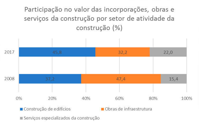
Em relação a 2008, houve uma mudança na estrutura do valor da atividade, com a construção de edifícios passando a ser o segmento mais representativo, enquanto obras de infraestrutura caíram para o segundo lugar. Os serviços especializados mantiveram o terceiro lugar, mas ampliaram sua participação no valor da indústria da construção.

Além disso, no período analisado, o setor público perdeu representatividade como cliente da indústria da construção, com uma perda de 11 pontos percentuais no valor das obras e serviços, de 42,7% para 31,7%. O segmento de obras de infraestrutura, cuja participação pública como cliente é historicamente maior que a dos outros, foi o mais afetado, caindo de 60,3% em 2008 para 52,4% em 2017. O setor público como demandante de construção de edifícios recuou de 27,2% para 20,7%. Já os serviços especializados em construção apresentaram uma diminuição relativa menor, saindo de 23,4% para 21,7%.

Média de pessoal ocupado e salário médio mensal da construção caem

As empresas da construção empregavam cerca de 1,91 milhão pessoas em 2017, sendo 37,1% na construção de edifícios; 35,0% em serviços especializados; e 27,9% nas obras de infraestrutura.

Em relação a 2008, as obras de infraestrutura perderam participação no pessoal ocupado e passaram do segundo para o terceiro lugar, sendo superadas pelos serviços especializados da construção. O segmento de construção de edifícios se manteve como o principal empregador ao longo da série.

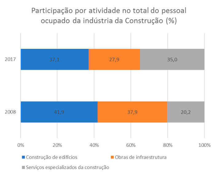
Além disso, houve uma queda na média de pessoal ocupado por empresa, que era de 32 pessoas em 2008 e passou para 15 em 2017. O salário médio mensal passou de 2,7 para 2,3 salários mínimos.

Todos os segmentos tiveram quedas na média de pessoal ocupado. O segmento que mais perdeu participação entre 2008 e 2017 foi de obras de infraestrutura, que tinha o maior porte médio (de 93 para 42) e a maior média salarial (de 3,5 para 2,9 salário mínimos). Como resultado, o perfil do emprego na construção passou a ser frequentemente relacionado a salários mais baixos.

Gastos com pessoal representam 33,8% das despesas da indústria da construção

O principal item de custos e despesas da atividade de construção, tanto em 2008 quanto em 2017, foi o referente aos gastos de pessoal, passando de 29,2% para 33,8%. O consumo de materiais de construção registrou queda de 26,6% para 22,0%. Por sua vez, as obras e/ou serviços contratados passaram de 10,7%, em 2008, para 9,1%, em 2017.

Entre os produtos e/ou serviços oferecidos pelas empresas com 30 ou mais pessoas ocupadas, os três grupos de produtos com maior participação no valor de incorporações, obras e serviços da construção foram: obras residenciais (24,3%); construção de rodovias, ferrovias e obras urbanas (18,8%); e os serviços especializados para construção (18,0%).

Participação da região Sul na indústria da construção foi a que mais cresceu

Entre 2008 e 2017, embora a região Sudeste tenha perdido participação, permaneceu liderando em pessoal ocupadas e valor das incorporações, obras e/ou serviços da construção. Por outro lado, a região Sul apresentou os maiores ganhos de participação, tanto em valor como em pessoal ocupado.

Na geração do valor de incorporação, obras e serviços da construção, a participação do Sudeste passou de 55,5% para 49,8%. A região Norte também perdeu participação (de 7,9% para 5,6%), enquanto Sul (de 12,1% para 17,1%) e Nordeste (de 15,8% para 18,9%) ganharam participação. Já região Centro-Oeste manteve sua participação estável em 8,7%.

A distribuição regional do pessoal ocupado na Indústria da Construção acompanhou o padrão do valor de incorporação, obras e serviços da construção. Entre 2008 e 2017, houve redução da participação do Sudeste (de 51,7% para 48,8%) e do Norte (de 6,7% para 5,6%) no pessoal ocupado, enquanto o Nordeste (de 19,9% para 21,2%) e, principalmente o Sul (de 13,5% para 16,3%), ganharam participação. A região Centro-Oeste manteve estável a sua participação no pessoal ocupado da Indústria da Construção no período.

Regionalmente, a pesquisa leva em consideração somente as empresas com cinco ou mais pessoas ocupadas.

Indústria da construção perde 93,6 mil trabalhadores e 564 empresas em 2017. Indústria da construção registra queda de pessoas ocupadas

A indústria da construção perdeu cerca de 93,6 mil pessoas ocupadas e fechou 564 empresas entre 2016 e 2017. No mesmo período, o valor gerado pelas incorporações, obras e/ou serviços caiu 9,6%, recuando para R$ 280 bilhões, em termos nominais. Os dados são da Pesquisa Anual da Indústria da Construção (Paic), divulgada hoje (29) pelo IBGE.

“O cenário de baixo crescimento, instabilidade econômica e incertezas institucionais tem desestimulado os investimentos, e o setor [de construção] perdeu dinamismo nos últimos anos”, analisa a gerente de Pesquisas Estruturais e Especiais do IBGE, Fernanda Vilhena.

De fato, nos resultados do Produto Interno Bruto (PIB) de 2017, o investimento, mensurado pela formação bruta de capital fixo, apresentou uma queda de 2,5%, sendo a construção o componente de maior peso.

Como exemplos na redução dos investimentos, Fernanda destaca os desembolsos em infraestrutura do Banco Nacional de Desenvolvimento Econômico e Social (BNDES), que, apesar do ligeiro aumento nominal em 2017, tiveram fortes retrações em 2015 e 2016. Além disso, o crédito imobiliário também apresentou queda intensa entre 2016 e 2017, com redução no número de unidades financiadas.

Boa parte dessa retração se refletiu no segmento de infraestrutura, que perdeu participação no valor das incorporações, obras e/ou serviços ao longo dos últimos anos. Por outro lado, a construção de edifícios ganhou representatividade. De 2008 a 2017, a participação do segmento de infraestrutura caiu de 47,4% para 32,2%, enquanto a da construção de edifícios cresceu de 37,2% para 45,8%.

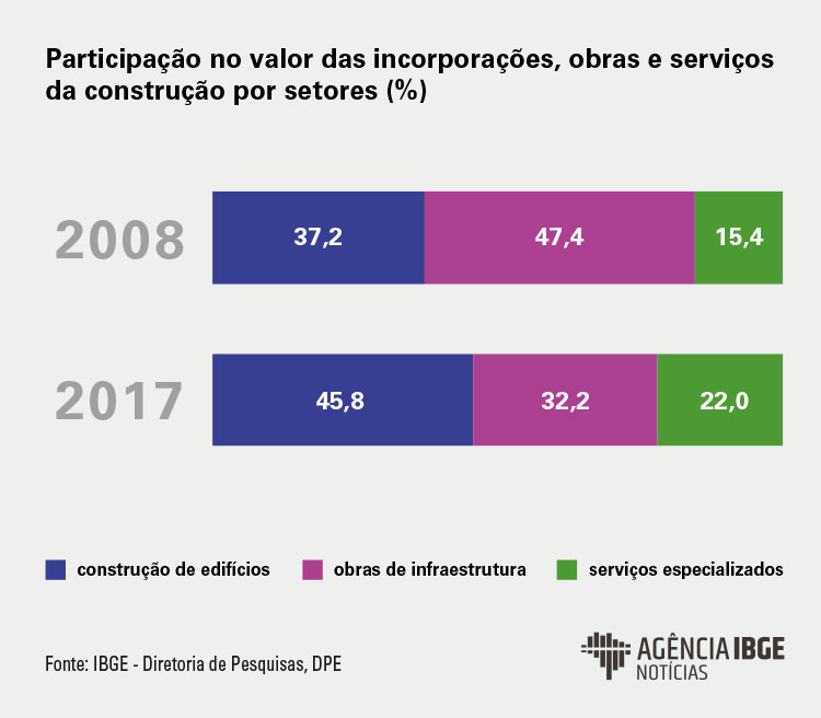
Fernanda explica que esses números vêm acompanhados da diminuição da participação do setor público como cliente na geração do valor de obras. “De 2008 para 2017, a participação do setor público caiu para a indústria como um todo, mas principalmente no setor de infraestrutura, que é muito dependente do investimento público”.

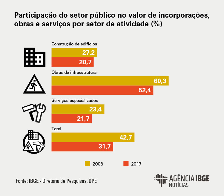
Pessoal ocupado na construção é o menor desde 2008

Em relação ao emprego, a indústria da construção empregava, em 2017, cerca de 1,9 milhão de pessoas, mostrando uma queda de 4,7% em relação a 2016. Este é o menor contingente de ocupados desde 2008, quando havia cerca de 1,8 milhão de pessoas ocupadas no setor da construção.

Todos os segmentos tiveram queda na média de pessoal ocupado. Porém, o segmento que mais perdeu participação entre 2008 e 2017 foi também o de obras de infraestrutura, que tinha o maior porte médio e a maior média salarial.

“Em participação no emprego, o segmento de infraestrutura foi superado pelos serviços especializados, que são empresas menores, de serviços de acabamento, pintura, encanamento, caracterizados por pagarem salários mais baixos. Ou seja, os empregos que ganharam participação foram justamente os associados aos salários mais baixos, mudando o perfil do emprego na construção”, conclui Fernanda.

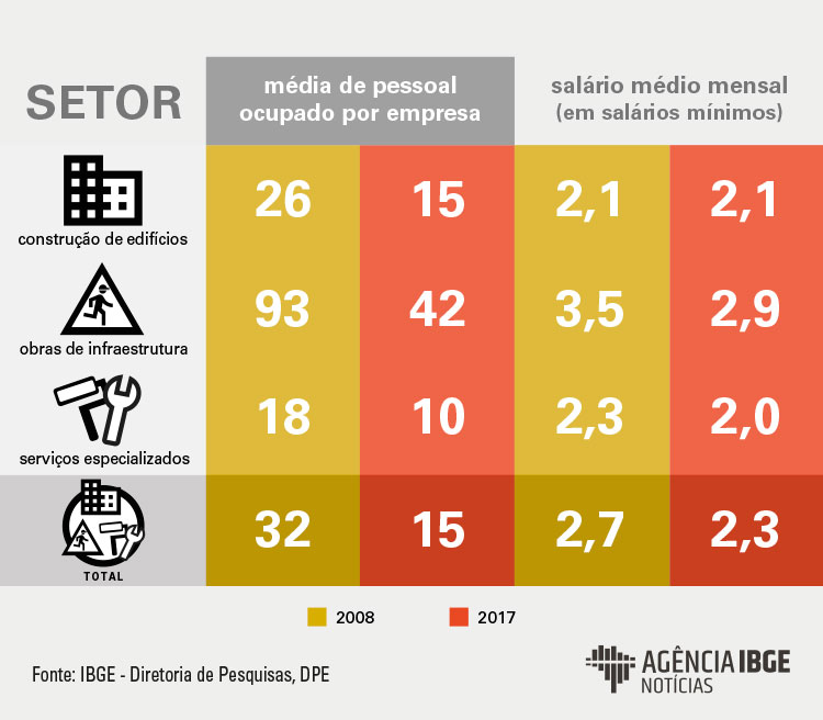
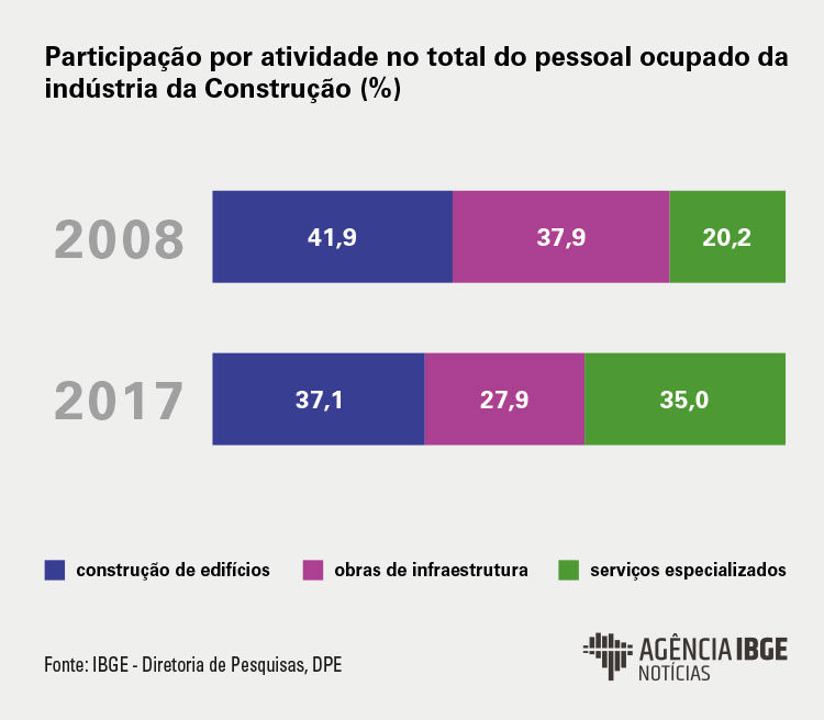
DOCUMENTO: https://agenciadenoticias.ibge.gov.br/agencia-sala-de-imprensa/2013-agencia-de-noticias/releases/24626-paic-2017-obras-de-infraestrutura-e-setor-publico-perdem-participacao-na-industria-da-construcao

_________________

LGCJ.: